Use the following steps to integrate the SFRA in the project:

1. To enable the SFRA functionality, the predefine symbol SFRA_ENABLE must be added in the project properties as shown in Figure 4-2.
2. To start an SFRA sweep, put the SFRA object in the watch window.
3. Write SFRA_OBJ.start to 1, when you want the SFRA sweep to start as shown in Figure 4-39.
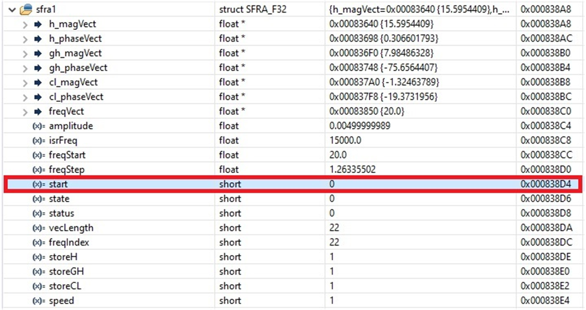   Figure 4-39 Start SFRA Functionality
4. Monitor the SFRA_OBJ.FreqIndex variable; the variable gradually increments as SFRA sweep is performed.
5. Once the SFRA_OBJ.FreqIndex reaches Vec_Length, the SFRA sweep is complete.
   Figure 4-40 SFRA Data Arrays
6. As part of the SFRA initialization, the Open Loop and Plant Magnitude and phase are stored in arrays called.

   __attribute__ ((section(".sfradata"))) float32_t plantMagVect[SFRA_FREQ_LENGTH];
   __attribute__ ((section(".sfradata"))) float32_t plantPhaseVect[SFRA_FREQ_LENGTH];
   __attribute__ ((section(".sfradata"))) float32_t olMagVect[SFRA_FREQ_LENGTH];
   __attribute__ ((section(".sfradata"))) float32_t olPhaseVect[SFRA_FREQ_LENGTH];
   __attribute__ ((section(".sfradata"))) float32_t freqVect[SFRA_FREQ_LENGTH];

7. Put these in the watch window to inspect and study the response.
8. Once the sweep is complete, click on View-> MemoryBrowser inside CCS.
9. Inside Memory Browser, enter &freqVect to see the frequency vector and select 32-bit floating point,
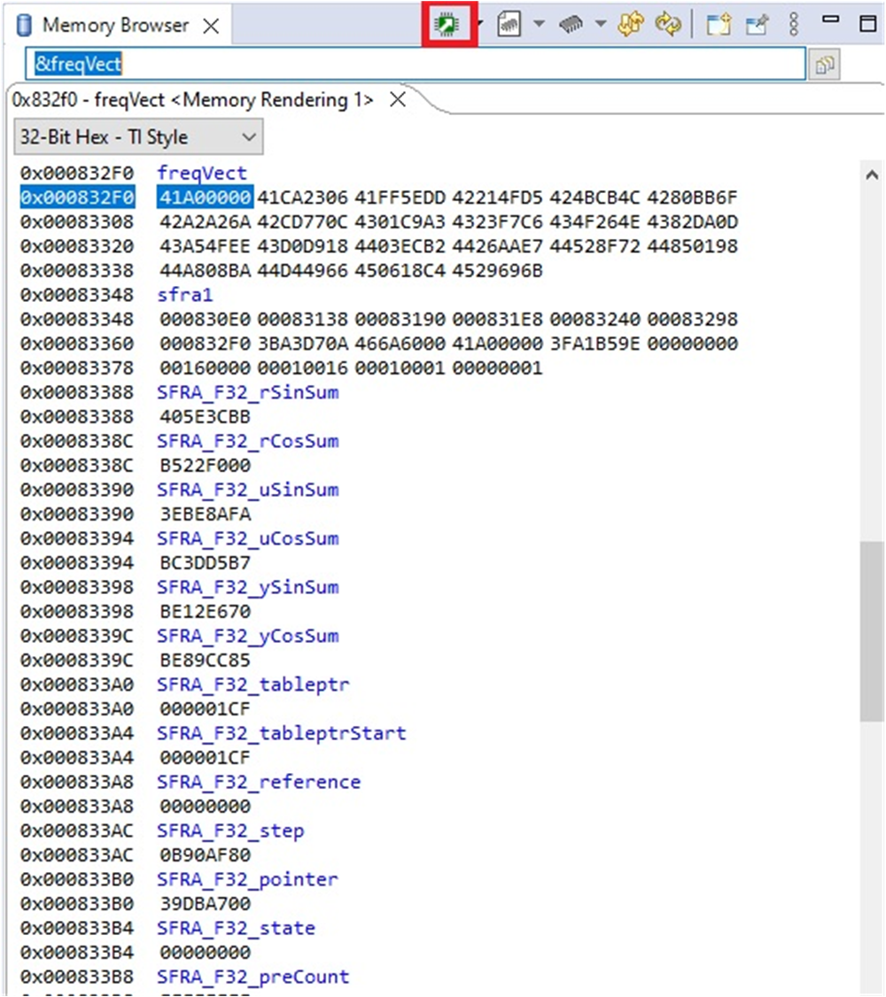   Figure 4-41 Memory Browser View of Stored SFRA Vectors
10. Click on save memory, shown encircled in Figure 4-41.
11. A pop-up window appears. Select TI data and specify the file name *.dat in the location you prefer.
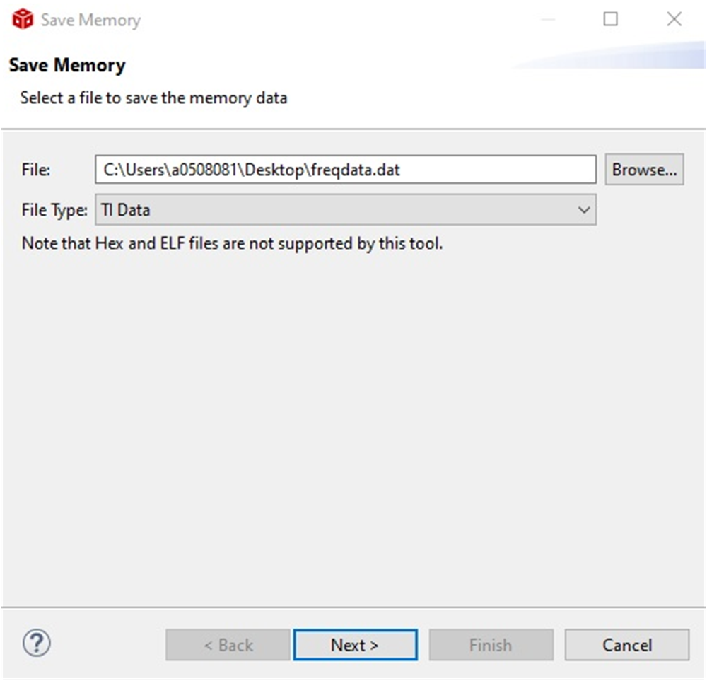    Figure 4-42 Save Memory Pop-Up Window
12. Click on Next and specify the address from the memory browser for the start of the array and then the length.
13. Make sure 32-bit floating point is selected. Click Finish.
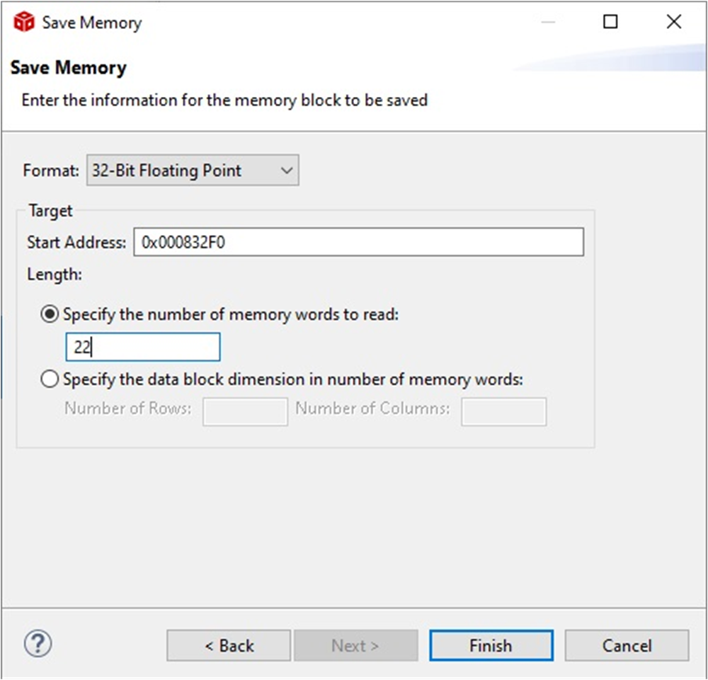    Figure 4-43 Save Memory Options
14. This saves the data in *.dat file.
15. Repeat this step for plantMagVect, plantPhaseVect, olMagVect, olPhaseVect, so you have 5 *.dat files.
16. If you want to use this data in MATLAB or other tools, the data can be populated to an excel file.
17. Open the SFRA.xlsx file located at <project directory>\libraries\SFRA\scripts in excel.
18. You can choose to re-name and save the file.
19. This excel sheet has five columns, in the first column is the frequency data.
20. Open the *dat file that was saved.
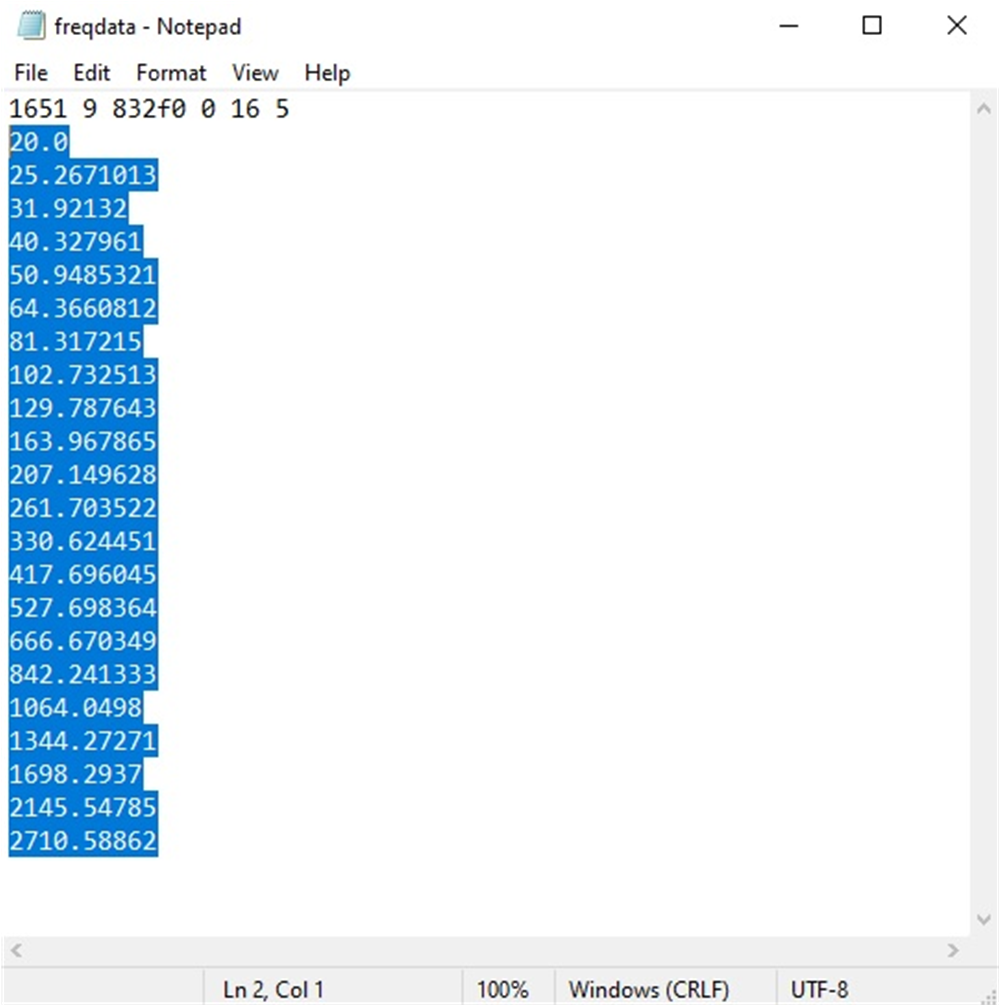    Figure 4-44 Selecting Data From .dat File to Put in the Excel
21. Select the data from the second line onwards to the end of the file and do Ctrl+C to copy the data.
22. Open the Excel File, go to the first element under the corresponding vector and do Ctrl+V to copy the array.
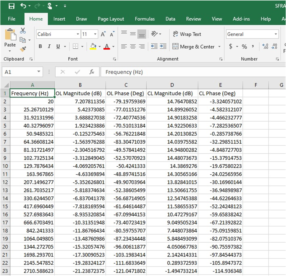    Figure 4-45 SFRA Data Copied in Excel File
23. Repeat the steps for each column.
24. Once the excel file is updated for all five columns, use the MATLAB script to import the SFRA data. Then, use the script inside sisotool to design compensator and carry out stability analysis.