The Ackermann steering model is commonly used throughout the automobile industry, to mathematically model the path that the tires of a car follow during a turn. As Figure 1-1 shows, the four tires follow a set of four concentric circles.

Figure 1-1 Ackermann Steering Curves

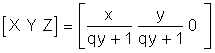
Given the wheelbase (L), tread (W), and inner tire steering angle (δ_i), the Ackermann steering model and the Pythagorean Theorem are used to determine the radius of the path of the front inner tire and the radii of the paths of the rear tires, as shown in Equation 1, Equation 2, and Equation 3. To generate the paths that the tires follow, in such a way that they can be mapped to a display, a conversion factor from inches to pixels must be applied before calculating the radii of the paths. The sample code in the Vision-SDK uses a conversion factor of 9 pixels to 1 inch.

Equation 1.

Equation 2.

Equation 3.

After finding the radii of the paths, the standard form equation of a circle can be used to generate the paths the tires follow. In the current implementation, for a given x value in the set xPathMin ≤ x ≤ xPathMax, the corresponding y value is calculated using Equation 4.

Equation 4.

Figure 1-2 and Figure 1-3 show the MATLAB outputs of a script which takes the inner tire steering angle (δ_i) and turning direction input, and then generates rearview curves using the previous equations. Figure 1-2 shows the rearview curve for a 0° steering angle, and Figure 1-3 shows the back up curve for a 45° steering angle left turning direction input.

Figure 1-2 Rearview Curve for 0° Steering Angle

Figure 1-3 45° Left Steering Angle

While the previous figures model the top-down view of the paths the tire follow, the rearview camera angle requires the rearview lines to appear to be converging to a finite vanishing point on the z-axis. The single-point projection transform manipulates the image such that points at infinity are mapped to a finite value in 3D space. In this case, the curves must be projected with respect to the y-axis, therefore Equation 5 was derived and used in the algorithm.

Equation 5.

Before the transform can be properly applied, the center point of the rear axle is mapped to the origin. Specifically, the curves must be translated so that the path of the driver-side tires is in the second quadrant, and the path of the passenger-side tires is still the tread length away from the driver side tire. Figure 1-4 shows the MATLAB output of the previous transform applied to the curve generated in Figure 1-3.

Figure 1-4 Projected Rearview Lines From Figure 1-3

Lastly, the curves are translated so that they are in the rearview camera viewing window. Figure 1-5 shows the display output of the TDA3X RVP running the surround view + rearview use case, with the dynamic rearview lines being drawn using the draw2D API included in the Vision-SDK.

Figure 1-5 Display Output of Algorithm Running on TDA3x

The Vision-SDK, from TI, contains a use-case generation tool which simplifies development by letting the developer quickly specify which algorithms run on which core, and in what order. Using the use-case generation tool, a new link was added to an existing use-case that displays 3D surround view and the rearview camera. The algorithm described in the previous section was implemented on the C66x DSP in the Alg_drawRearview link. Figure 2-1 shows the use-case flow chart generated from the output of the use-case generation tool. Additional documentation on the link and chain structures and use-case generation tool is in vision_sdk/docs.

The AlgorithmLink_drawRearviewCreate function is called when the use-case is instantiated. The necessary link parameters for the links and chains framework are generated with this function. This includes allocating the memory and initializing the input and output queues, setting up the output color format, the required buffer information for the draw2D API, and the data structures used within the algorithm link.

Next, the link architecture invokes the AlgorithmLink_drawRearviewProcess function using a notification generated by the previous link, indicating that the input queue is ready to be processed. The use-case architecture requires the rearview lines to be drawn at the same frame rate that is output to the display. However, the current implementation of the Alg_drawRearview link calculates the discrete points on the rearview curves at a rate of 15 frames per second (FPS) and stores them in a buffer that is drawn at a rate of 30 FPS.

Figure 2-1 Dynamic Rearview Lines + 3D Surround View Use-Case Links and Chains Flow Chart

The Alg_drawRearview function leverages the draw2D API to draw the rearview lines on the video frame. This occurs within the AlgorithmLink_drawAckermannSteering function, where the discrete points of the rearview lines are calculated and drawn, based on the steering direction and inner wheel steering angle. The function stores the coordinate pairs of each discrete point in a set of buffers, and then calls the Draw2D_drawLine function to draw a line segment between two adjacent points. Draw2D_drawLine has a line parameter struct input that lets the developer set the color format, color, and thickness (in pixels) of the lines drawn.

Currently, the dynamic rearview lines demo in the Vision-SDK is a proof of concept that uses a switch statement to update the steering angle and steering direction each time the AlgorithmLink_drawRearviewProcess function is invoked. In an application where a steering wheel is available, the developer could implement a CAN BUS monitor link and a data sync link that could aggregate the steering wheel input data with the video frame that has the same timestamp into the input queue of the Alg_drawRearview link. The data could then be parsed in the AlgorithmLink_drawRearviewProcess function and the AlgorithmLink_drawAckermannSteering function could be called to generate and draw the rearview lines.