4 Case-Study-1: Motion Classification

Radars natively have very good velocity resolution. A machine learning backend enables the radar to recognize motion signatures. This can be leveraged in many applications that can benefit from the classification of tracked objects.

Figure 4-1 is a representative signal processing chain for motion classification. The received ADC data is first processed using traditional FFT processing (Range-FFT, Doppler-FFT, Angle-FFT) to generate a radar cube. Next, a detection layer identifies peaks and generates a point cloud. The point cloud is then clustered into objects using a multi-target group tracker (perhaps based on an Extended Kalman Filter). µ-Doppler spectrograms are then generated for each tracked object. The centroid for each tracked object is mapped to the corresponding location in the radar-cube and a µ-Doppler spectrum is extracted from the neighborhood of this centroid. The µ-Doppler spectrum is concatenated across multiple consecutive frames to generate a µ-Doppler vs. time heatmap. This can be sent to a 2D-CNN for classification. Alternatively, a hand-crafted feature extraction block can be implemented to create a 1D time sequence data from the sequence of spectrograms, which can then be classified using a 1D-CNN. This has much less complexity than a 2D-CNN.

In our study, the above approach was used to discriminate human vs. non-human motion [4]. This problem is relevant in indoor and outdoor surveillance, where discrimination between motion from humans and other sources such as pets, trees, fans, etc. prevents false alarms. A total of six features (upper and lower envelopes, mean and median, normalized bandwidth, and normalized spectral entropy) are extracted from µ-Doppler to be used by the classifier. The feature extraction is repeated for consecutive frames within a sliding window, whose size is determined based on the tradeoff between the classification accuracy and the latency. In this study, a typical block length of 20-40 frames (2-4 sec @10 Hz) is used. We then build and train a 1D-CNN model to classify the target objects (human or non-human) given the extracted features as time series data.

The 1D-CNN architecture is shown in Figure 4-2. The input size is configured as the total number of features. Two blocks of 1D convolution, ReLU, and layer normalization layers are used, where the convolutional layer has a filter size of 3. To reduce the output of the convolutional layers to a single vector, a 1D global average pooling layer is added. To map the output to a vector of probabilities, a fully connected layer is used with an output size of two (matching the number of classes), followed by a softmax layer and a classification layer. As illustrated in Figure 4-2, an optional block of 1D convolution with 64 filters, ReLU, and layer normalization layers (following the first two blocks) is also added to compare the performance of 2 vs. 3 layers CNN models

In the experimental results, a total of 125816 frames of data were captured at 10 Hz (corresponds to 3.5 hours in total) from different human and non-human targets. In the data capture campaign, 310 scenarios are created in distinct environments with around 20 different people and numerous non-human targets (e.g. fan, tree, dog, plant, drone, etc.). The data is captured with synchronized video to assist in labeling. In total, 31611 observations (14901 human, 16710 non-human) are generated when the time window size is configured to 20 frames (2 sec at 10 Hz), and 2 frames stride is applied to allow the changes in the statistics.

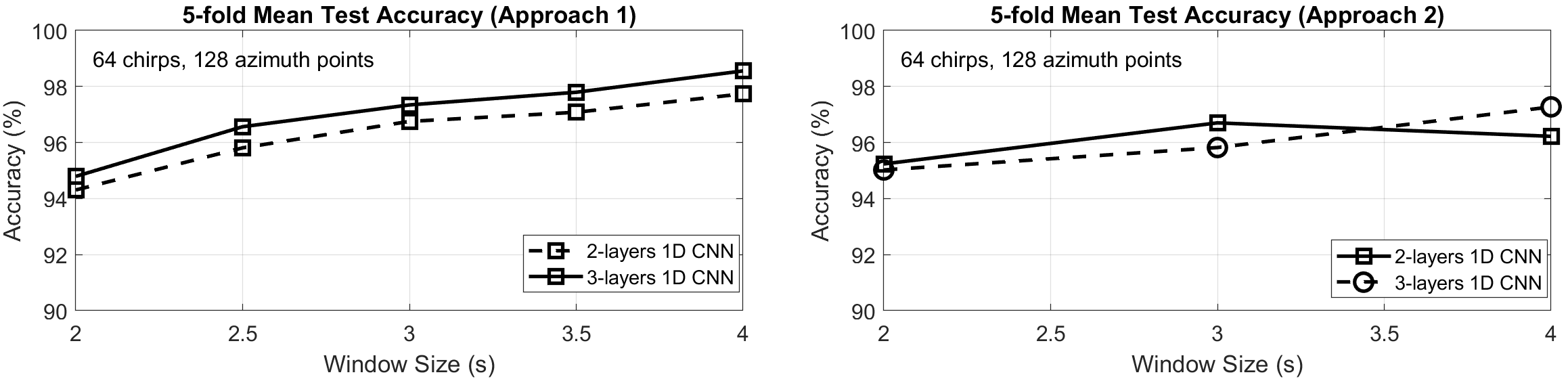
The performance of the classifier was characterized using two approaches. The first approach uses all the available data combined, shuffled, and split as follows: 40% for training, 10% for validation, and 50% for test. The second approach reserves some specific portion of the data set for testing, consisting of human and non-human subjects that were completely absent from the training set. With either approach, the overall classification error is calculated using 5-fold cross-validation. For each iteration (i.e., fold), data is reshuffled, and the accuracy is calculated with different random combinations of training, validation, and test data. The average of the test accuracies obtained from each iteration is then reported as the final accuracy metric. Figure 4-3 summarizes the performance of the first and second approaches, respectively. These results show that the proposed 1D-CNN classifier can achieve about 95% average accuracy in challenging test scenarios even with a 2 sec window and 2 layers.