SBAA632 April 2024 TMAG3001 , TMAG5170 , TMAG5170-Q1 , TMAG5170D-Q1 , TMAG5173-Q1 , TMAG5273
2.1 Build Configuration
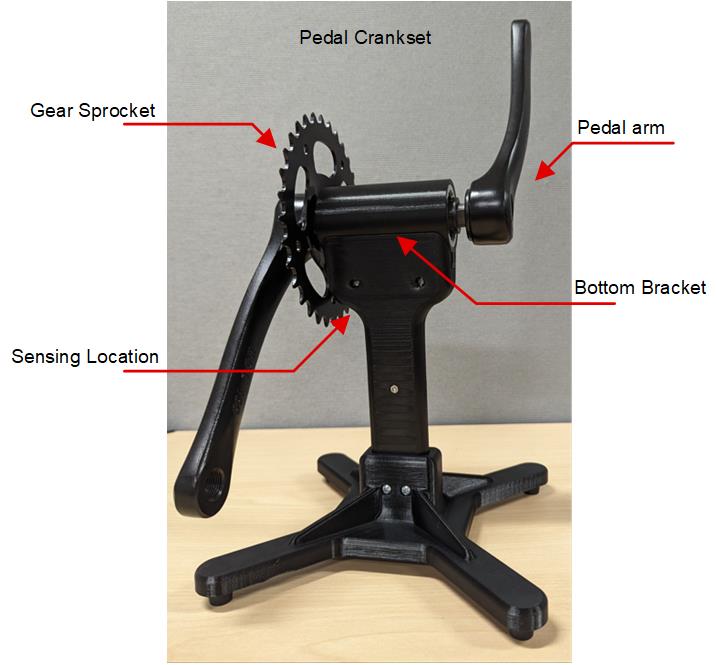
To demonstrate this behavior, a 32-tooth crankset and bottom bracket were mounted into a 3D printed assembly.
 Figure 2-1 Gear Tooth Sensing
Setup
Figure 2-1 Gear Tooth Sensing
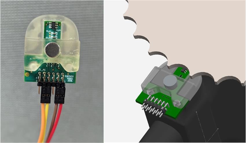
SetupA bracket to mount either the TMAG3001 (a small commercial grade 3D sensor in a WCSP package) or TMAG5173-Q1 (an automotive grade 3D sensor in a small SOT-23 package) with a back bias magnet was designed to position the sensor in near proximity to the rotating front sprocket. On this demonstration there is no chain, but in a practical setting this needs to be installed on the section of the sprocket where the chain does not rest.
 Figure 2-2 TMAG5173-Q1 Sensor and
Back-bias Magnet Placement
Figure 2-2 TMAG5173-Q1 Sensor and
Back-bias Magnet PlacementFor most riders, a pedal speed of 80-100 RPM is considered a designed for target when riding unassisted. Speeds above 110 RPM are typically only achieved during sprints. Suppose a target maximum speed of 150 RPM is set using a 32 tooth gear. In this case, the transit time for each tooth has a time span of approximately 78ms. In this case, we can calculate a desired sample rate based on the number samples per tooth.
While the Nyquist rate can require only 2 samples per oscillation as a minimum to detect each tooth, it is typically desirable to sample at a higher rate to gather a more complete profile. Consider below what is observed for the Nyquist rate compared to sampling 5 times per oscillation. In the case shown in Figure 2-3, the sampling is aligned to each zero-crossing and to the peak values. With any skew from this unique case, there can always be at least 2 samples per half cycle of the sine wave.
 Figure 2-3 Sampling Rates
If 5 samples are used in each 78ms time period, then approximately 15.6ms are available between each sample. To measure cadence with both speed and direction information, using a 3D Hall-effect sensor is helpful. TMAG3001 and TMAG5173-Q1 each are able to sample 2 axes needed for angle sensing in about 75us per sample. Averaging can be enabled to reduce the impact of noise on the end result at the cost of longer integration times. These sensors can average up to 32x per sample, with an effective sample time for two axes near 1.625ms. However, the recommendation in this particular application to not set the averaging higher than is needed. Since the tooth is moving during the duration of the sample period, a high degree of averaging produces unnecessary system delay. Data collected in this report used 8x averaging to limit angle noise.